
Introduction
 Inverted Pendulum (or Cart and Pole) Inverted Pendulum (or Cart and Pole) |
Fuzzy logic systems have been seen by many to be an alternative method of control, to more classical approaches, such as PID controllers. The main advantage of fuzzy controllers is there ability to cope, to a certain degree, with changes in the system being controlled. This ability usually comes at the cost of accuracy when compared to conventional controllers.
This report discusses the use of an Evolutionary Algorithm (EA) as a method to improve the accuracy of a Mamdani fuzzy controller. The motivation behind this approach is to find a technique, which could be used to optimise any fuzzy controller to improve accuracy. Thus, to produce a controller which is able to cope with certain changes in the system with the benefits of fuzzy logic, such as linguistic interpretability and the accuracy of conventional controllers.
The following chapter introduces fuzzy control systems and gives a evaluation of different fuzzy methods and more conventional approaches to control. This is then preceded by a review of different techniques currently used to optimise fuzzy controllers. Chapter 3 describes EAs and how they could be used in optimisation. This is followed by a brief description of the inverted pendulum problem and the Mamdani controller implemented. Chapter 5 reviews the EA implementation and justifies design decisions made. An analysis of the results obtained from using the EA is then presented. This is followed by a conclusion, which evaluates the effectiveness of the EA as a means of optimisation.
Fuzzy Control Systems
A Fuzzy control system is a control system implemented using fuzzy logic. The majority of fuzzy control systems are based on the Mamdani model or an extension of this such as the Takagi-Sugeno model.
Fuzzy control has been used in many industrial systems since the late 1970s. More recently fuzzy control has been used in a number of commercial products such as electric shavers, automatic transmissions and video cameras, Russell and Norvig (2003) review a number of these commercial systems and note that a number of papers argue that, these applications are successful because they have small rule bases, no changing of inferences, and tuneable parameters that can be adjusted to improve the system’s performance. “The fact that they are implemented with fuzzy operators might be incidental to their success” (Russell and Norvig, 2003).
Two widely used fuzzy system types are Mamdani and Takagi-Sugeno. These types differ in their methods of rule consequent. The Mamdani system uses an output membership function with defuzzification techniques to map the input data to an output value. The Takagi-Sugeno system, as described by Zimmermann (2000), uses the same fuzzy inference as the Mamdani method, only differing in the way in which the rules are processed as it uses functions off the input variables as the rule consequent. The Takagi-Sugeno method is often used to implement control systems, where the Mamdani method is usually used for handling information, such as sorting data into classes.
This report will be focusing on using the Mamdani method to create a control system, although it is known that this may not be the best solution.
2.1. Alternative to Fuzzy Controllers
An alternative approach to controlling the fuzzy pendulum is to use a PD controller, an implementation for which is provided in the MATLAB Toolbox as a four-term linear controller. This controller would be classed as a PID controller if an integral were used to track errors over time. The PD controller is based on equations, which calculate an estimate of the proportional and the derivative parts. These values are then tuned to find optimal values, by testing the controller and making adjustments of the proportional and derivative parts based on the output of the system. PD controllers are designed using mathematical equations, which are used to produce control functions based on a model of the system.
2.1.1. PD and Fuzzy Controllers
It is difficult to compare classical control and fuzzy control methods, as there construction is vastly different. Many designers of control systems prefer classical control methods, as they are based on mathematical equations, which can be manipulated to produce precise results. Whereas advocates of fuzzy control are keen on the linguistic interpretability, with respect to changing and understanding the effects of the system based on structured words.
Fuzzy controllers have been shown to be an alternative and in a number of cases a better method of control compared to more classical methods of control such as PD and PID controllers. A number of studies, reviewed by Mamdani (1981), identify advantages of using these fuzzy controllers. “many studies have found that this type of controller is more robust to plant parameter changes than a classical controller”. These advantages describe the ability of fuzzy controllers to handle varying changes in the systems, Mamdani suggests, “this is merely the consequence of using heuristics. Human experience, which these heuristics amount to, is by nature robust” (Mamdani, 1981). More recently, Mohagheghi et al (2005), has described a weakness of classical control in handling changes in system characteristics, “The drawback of such PI controllers is that their performance degrades as the system operating conditions change.” (Mohagheghi et al, 2005).
PD and PID controllers require a model of the system. With this model the parts of the controller can be identified and an approximation of the controller can be produced, with further testing, the controller can be tuned to produce a near optimal controller. This technique is a proven and widely accepted method for producing system controllers. This technique however, requires a model of the system to be available. “Conventional (non fuzzy) control systems are designed with the help of physical models of the considered process. The design of appropriate models is time consuming and requires a solid theoretical background of the engineer” (Zimmermann, 2000). This indicates that in certain situations, if a model of the system is already available, then a PD or PID controller may be less time consuming to produce then a fuzzy controller, and if a model is unavailable then a fuzzy method may be more applicable.
2.2. Optimising the Fuzzy Controller
When designing a Mamdani fuzzy controller various techniques are used. These techniques, in the most part, use heuristic methods to make a ‘best guess’ of what the rules and membership functions should be. Zimmermann (2000) describes various methods for constructing fuzzy controllers, the majority of which use a heuristic approach to approximate what the ‘best’ values could be. These methods usually result in a sub-optimal controller, which needs to be tuned by trial and error in order to produce a controller, which works as well as possible.
The amount of system information available to the designer can have a direct impact on the quality of the controller, with more information resulting in a better performing fuzzy controller. However, this information can rarely be used to model the system exactly, so optimisation techniques should be used. “even information available on the behaviour of the plant does not necessarily lead to optimal fuzzy controller parameters; therefore the parameters of the fuzzy controller should be adapted in order to ensure an optimal performance” (Mohagheghi et al, 2005).
2.2.1. Optimisation for changing systems
Often in control systems, the characteristics of the entity being controlled changes in some way. This can be an issue, as the controller is no longer performing optimally. Fuzzy controllers, due to their ‘fuzzy’ nature are able to handle these changes to the most part, however only to a certain degree of change. “the main drawback of the conventional fuzzy controllers is that their control parameters are fixed and are not adaptively updated to adjust to the system operating conditions changes, sensors/equipment aging and suchlike.”(Mohagheghi et al, 2005).
A method sometimes used for optimising fuzzy systems is with the use of an evolutionary algorithm, Lee and Takagi (1993) addresses the problem of learning membership functions with evolutionary algorithms. In their approach the set of rules is defined a priori and the GA is used to optimise the shape of the membership functions. Another approach described by Bonari (1996), is ELF (Evolutionary Learning for Fuzzy rules), which uses evolutionary learning techniques such as genetic algorithms and learning classifier systems to learn fuzzy rules.
Other often-used techniques are gradient ascent/descent and artificial neural networks. Both techniques have a number of advantages and disadvantages. This report will focus on the use of evolutionary algorithms as the method of optimisation, which is introduced in the next chapter.
Evolutionary Computation
Evolutionary algorithms can be divided into two main areas of research. These are genetic algorithms and evolutionary strategies. Both areas share many similarities and the majority use the genetic operators, mutation, crossover and selective reproduction in order to evolve a population to produce a new generation. “The essential ingredients in any evolutionary algorithm are population-based random variation and selection.” (Fogel, 2000). As the division between the two areas is not clearly defined, the general term, evolutionary algorithm, will be used, which encapsulates both these approaches.
Evolutionary algorithms are an often-used technique for optimisation problems where the performance of the system cannot be used to identify what needs to be improved. The main strengths of an evolutionary algorithm is the ability to search a large number of diverse possibilities, with only the need of a single evaluated value indicating how well a particular solution performed.
Evolutionary algorithms are often chosen as a more efficient method to other techniques such as gradient ascent/descent. “Because of their universality, ease of implementation and fitness for parallel computing, EAs often take less time to find the optimal solution than gradient methods.” (Sbalzarini et al 2000). One crucial difference between evolutionary algorithms and more classic methods such as gradient search is these will produce the same solution time again, whereas the evolutionary approach can often result in solutions with subtle differences, due to the nature of using random functions. Mitchell (1998) describes a common application of evolutionary algorithms, ‘where the goal is to find a set of parameter values that maximise a complex multi parameter function’.
The following chapter introduces the pendulum problem and describes, the steps taken to produce a fuzzy controller using the Mamdani method. An evolutionary algorithm is then introduced as a method of optimising the Mamdani controller.
Inverted Pendulum Problem
The inverted pendulum or cart and pole dilemma is a problem often used for benchmark testing different control methods. The problem involves balancing an inverted pendulum, while following a desired location marker. The aim is to move the pole to its destination smoothly without overshoot and as quickly as possible.
4.1. Mamdani Fuzzy Controller
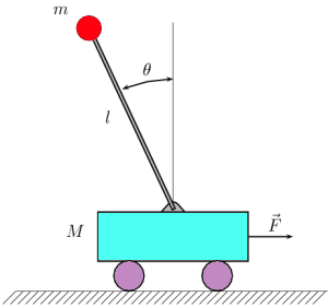
A Mamdani fuzzy controller has been implemented here to balance the inverted pendulum, designed using the fuzzy inference tool for MATLAB. As the input and output space of the Mamdani method is based on membership functions, the scope of design can be rather limited. Figure 1 shows a diagram of the inverted pendulum problem, the labels and arrows show the distance and direction of the four readings that are available as inputs to the fuzzy controller.
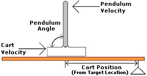 Figure 4.1 – Inverted Pendulum Problem Figure 4.1 – Inverted Pendulum Problem |
From the diagram shown in Figure 4.1, the rules for the fuzzy controller can be deduced. The four rules chosen, shown in Appendix A, are used in two complementary pairs, one pair keeps the pendulum upright and the second pair moves the cart to the target position.
To move the cart to the desired location and keep the pendulum balanced, involves forces being applied to the left and right sides of the cart. The rate and strength of these forces need to be considered with attention being made to the following:
- How much freedom the pendulum has, with respect to the minimum and maximum angle allowed.
- How fast the cart should move (has a direct effect on how quickly the cart arrives at the target location)
- How much the cart is allowed to overshoot the target location
4.2. Robustness of Approach
The implementation of the Mamdani fuzzy controller involved much trial and error. Although the rules were found by analysing the system, the values and range of the membership functions were, for the most part, based on an educated guess of the effects too large and small values could have on the system. The process of essentially ‘guessing’ the membership set values, seems to indicate that this could be done with an automated process, of evaluating each change made until an acceptable solution is found.
As mentioned in chapter 2, a Mamdani controller may not be best suited for control applications. A better fuzzy method would be a Takagi-Sugeno system, which is often used in control systems based on fuzzy logic. Thus a comparison of the Mamdani and Takagi-Sugeno controllers will not be made here, as the direction of this report is towards the concept of optimising the Mamdani fuzzy controller with the use of an evolutionary algorithm. The inverted pendulum problem is being used, as it is an effective way of visually showing if the fuzzy system is approving over time. The fact that the Mamdani system is being implemented as a controller is not the main issue. The resulting algorithms and techniques learned from this report could be applied to a case more suited to a Mamdani controller, such as data mining. In theory the algorithm could also be extended to a Takagi-Sugeno system, by removing the output membership space control from the EA.
The following chapter describes the approach used to optimising the Mamdani fuzzy controller.
Optimising Fuzzy Controller with Evolution
Evolutionary algorithms (EAs) have been used in a number of systems requiring parameter optimisation. One such example, described by Mohagheghi et al (2005) uses a genetic algorithm to optimise a fuzzy controller for a static compensator used in power systems. The controller is reported as being more fault tolerant than the previous used PI controller.
An artificial neural network (ANN) is another approach often used in optimising fuzzy controllers, however they will not be used here, as they are notoriously difficult to inspect and understand the current internal state. With an EA each part of the process can be revealed.
Bonari (1996) reviews a number of cases where EAs have been used to optimise a fuzzy system, he notes that all the cases either define the rule base prior to optimising the membership functions or define the membership functions and use an EA to create the rules. There is no indication given of which is best, so it must be assumed that the decision is made on a case-to-case basis. The EA being designed here will be used to optimise the membership functions, the rule base will remain the same throughout. This decision was made, as it is evident from using the controller that it is capable of balancing the pendulum and moving in the correct direction. This indicates that the rules must be right. Another reason the EA is not being used to create the rules, is an EA would have know concept of readability, so a set of rules could be produced that worked, but were so complicated that they were not interpretable to the user, which is one of the benefits of using fuzzy logic.
The evolutionary algorithm will be designed for two purposes. Initially it will be used to optimise the existing Mamdani fuzzy controller, described in chapter 4. The second use will be to run the EA in order to adapt the controller to changes in the properties of the system. The following sections review the implementation of the EA produced, detailing the techniques used for evaluation, selection, crossover and mutation. A number of alternatives are shown, which in a few cases are described as better methods, which could be implemented in the future. For the implementation, the phenotype is the fuzzy controller, the population is set to 10 and the generation refers to an evolved population.
5.1. Fitness Evaluation Function
A fitness function is a key design issue in evolutionary algorithms and is used to evaluate how well a solution performed. A fitness value is an evaluation of each phenotype in the population and is used exclusively to determine the likelihood of the phenotype to reproduce. “The fitness function is a performance criterion that evaluates the performance of each individual phenotype” (Nolfi and Floreano, 2000). From reviewing the literature it seems that there are no proven techniques for designing a fitness function. The fitness function was used to evaluate how well the fuzzy controller performed in maintaining the pendulum inverted and moving it to the target location.
The implementation, the code of which is available on request, involved a number of steps. The first was to record the output of the MATLAB Simulink simulation of the inverted pendulum. This output is in the form of a table of data, which is made up of the four input values to the fuzzy controller sampled at regular time intervals. This data is saved in the MATLAB workspace and made available as a multi-dimensional array. Evaluating each piece of resulting data one-by-one would have been computationally inefficient; hence the fitness function first averages the data of each input and produces four values. These four values are then all made positive as what often happened was the pendulum would spin in one direction and the cart would move in a different direction, which resulted in two inputs having negative values and two having positive, which when summed would produce a low number. These four values are then added together to produce a single fitness value, with a value of zero being the fittest.
An issue arrived after testing the EA in simulation, this was that if the fuzzy controller was evolved in such away that the pendulum did not move at all, then no data would be produced from Simulink to show the distance the cart was from the target location. This could possibly have be an issue with the simulation, not producing results until the pendulum moved. To overcome this problem, first the minimum range and minimum membership function constraints were raised, which had no effect. The second approach, borrowed from reinforcement learning, was to use an offset value, which ‘punished’ the phenotype if the fitness value was exactly 0. This was an effective solution.
5.2. Selection, Crossover and Mutation
Selection and crossover are the compliments used in selective reproduction. This process involves choosing those individuals from the population, which have the ‘best’ chance of being combined to create a fitter generation. Two approaches to selective reproduction are the ‘Roulette Wheel’ and ‘Rank Selection’. “Selective reproduction is often implemented with the roulette wheel method, where each slot corresponds to an individual in the population and the size of the slot is proportional to the fitness of the individual.” (Nolfi and Floreano, 2000). This type of selection should select higher fitting phenotypes on average more of the time. The second approach, described by Zimmermann (2000), is to select the two highest fitting phenotype, apply crossover and then select the next two highest fitting phenotype and so on. Both methods apply crossover to half of the population and discard the least fitting members.
The method used for the implemented EA was similar to the ‘Rank Selection’ approach. First the highest fitting phenotype were selected and crossed over with any of the highest fitting half of the population, excluding the phenotype selected. This method was chosen as it was more computationally efficient than the ‘Roulette Wheel’ approach and was more scalable than the ‘Rank Selection’ technique, which, as reported by Zimmermann (2000), often produced a population favouring one or two individuals. The crossover procedure used, takes the two selected phenotypes and uniformly crosses a single random input/output membership set in order to create two new phenotypes, with a difference of one input/output membership set. A uniform crossover was used to enforce the constrained values, which are chosen for each of the four inputs and the output.
Mutation involved using random values, within a constrained range, to alter the membership range and membership functions of a randomly chosen input or the output. The rate of this mutation could be adjusted by specifying a larger upper range in the random selection of the input/output set to mutate, a value of 1-5 (4 Inputs, 1 Output), would result in a definite mutation, whereas a value of 1-10 would set the probability to a 50% chance of mutation for each member of the population.
5.3. Stopping Evolution
It was important to have a method of stopping the evolution process, in order to use the fuzzy controller being optimised. A number of methods were considered for this function. The first consideration, described by Nolfi and Floreano (2000), repeats the generation process until the best fitness value in the population stops increasing. This seemed a good solution to the problem, however it was noticed during initial testing, that it was common for the same high fitness value to be produced many times, which if this method were used, would stop the evolution with a sub-optimal solution. A second approach, which was implemented, used a fitness value of the fuzzy controller, detailed in chapter 4. This value was used as a ‘bench mark’ value. If a phenotype were produced with a lower fitness value, then the evolution would stop.
Another method considered, which was unfortunately not implemented due to time limitations, is described by Fogel (2000), in this method the phenotype with the highest fitness function, the ‘elite’, is stored in memory, until either a higher fitting phenotype is found, in which case the current ‘elite’ is overwritten or a maximum generation value is reached, where in which the ‘elite’ is regarded as the optimal solution in that instance. This method would present the best solution found in a predefined time scale.
5.4. Implementation Specifics
The code for the implementation of the EA is available on request. This code is designed to run in MATLAB as a completely automated process. Executing the ‘MATLAB_Evolution.m’ file starts the program running. The main elements of the code are:
- Creating, Reading and Writing ‘.fis’ files
- Crossover and Mutation
- Adjusting membership set ranges and point values
- Testing in simulation
- Fitness Evaluation
As this shows the components involved in the evolutionary algorithm for optimising the fuzzy controller, were: MATLAB Pre-defined functions, The Fuzzy Toolbox, Simulink, C functions converted to MATLAB extensions and ‘.m’ files to connect all of the operations together.
Analysis of Results
In the context of these experiments the phenotype is the fuzzy controller. The fitness value, is a measure of how well the controller performs in balancing the pendulum and moving to the desired location, the lower the value denoting a more stable system. Each trial uses a population of 10, initially random phenotype in 5 second simulations.
6.1. Mutation Rates
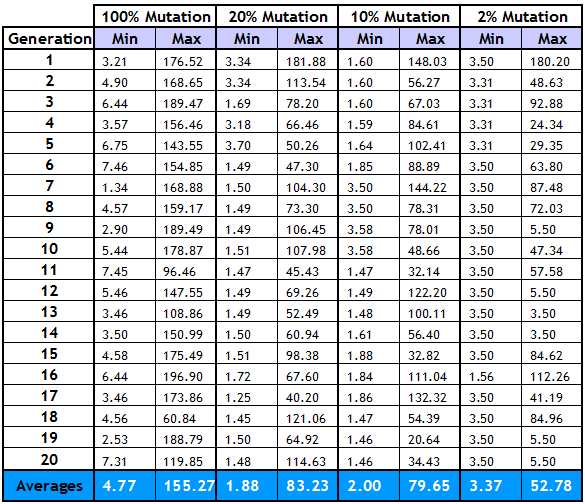
A number of different mutation rates were tested, to show how this rate effected the generations. These results are shown in the graphs of Figure 2 and are based on 20 generations averaged over 10 trials, using four different mutation rates. The table of results is provided in Appendix E. A mutation rate of 100% means that after crossover every element of the input and output is mutated for each phenotype, rates lower than this mutate fewer elements.
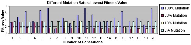 Figure 6.1 – Lowest Fitness values of four Mutation Rates Figure 6.1 – Lowest Fitness values of four Mutation Rates |
 Figure 6.2 – Highest Fitness values of four Mutation Rates Figure 6.2 – Highest Fitness values of four Mutation Rates |
Comparing the two graphs in Figure 6.1 and Figure 6.2, it can be seen that with 100% mutation more higher and less low fitness values are produced compared to generations using a lower mutation rate. It should also be noticed that with 100% mutation, low fitness values are lost between generations. Comparing the results of the lower fitness values, that the less mutation that takes place, the more chance the ‘best’ phenotype is reproduced in the next generation. It can also be seen that using a mutation rate of 2% can cause premature convergence, this is the result of crossover continually crossing the best phenotype, producing similar phenotype, without mutation these cannot be changed, thus crossover stops producing new generations which can outperform the ones previous. By using a high mutation rate and not mutating the highest fitting phenotype, it may be possible to preserve the best for future generations, until better performing phenotype are found. This could be the subject of future work.
6.2. Optimising the Fuzzy Controller
The EA was able to balance the inverted pendulum in an average of 6.3 generations over 10 trials this equates to 315 seconds of simulation, see Appendix B for table of results. The way in which the pendulum moved to the target location varied a considerable amount for each balanced pendulum. Many attempts moved passed the target location and many did not reach the target in the 5 seconds of the test.
These trials show that the EA is able to produce a fuzzy controller capable of balancing the inverted pendulum in a relatively short amount of time. However, the ‘quality’ of each controller varied significantly and thus no controller was found that could out perform the fuzzy controller constructed in chapter 4 (Appendix A). There are many reasons why an optimal fuzzy controller was not found. The first is that, it is difficult to evaluate each controller from its outputs, when these outputs are made up of four sets of 5000 results. The evaluation function used an average of each set of 5000 results, which was unable to take into account any patterns or changes of positive and negative values, which may signify subtle changes of the operation. A second issue, related to the first, is that stopping the evolution relied on finding a fitness value lower than that being optimised. A problem being that if the fitness value was flawed due to the output not being processed adequately by the evaluation function, then the EA would be searching for an inferior phenotype. A solution, which could improve the quality of the controllers produced, has been described in chapter 5.3. This involves storing the ‘elite’ phenotype and running the evolution for a predefined number of trials. This would mean that the highest fitting phenotype, found during any trial, would be presented at the end, instead of possibly being lost or mutated throughout the generations.
Conclusion
This report has explored the use of a Mamdani fuzzy controller to solve the inverted pendulum problem. The first part of this report involved producing a fuzzy controller using traditional heuristic methods. This was shown to be a good approach for choosing the rule base, however deciding on the membership function sets proved to be much more difficult. An Evolutionary Algorithm (EA) was introduced to choose the membership function set values that produced an optimal fuzzy controller for the purposes of balancing the inverted pendulum. The evolutionary algorithm was used to essentially optimise the existing fuzzy controller, using randomly constrained values for each point of the membership values and the range. The aim was to produce a controller with the linguistic interpretability of fuzzy logic, with the accuracy of a traditional PD controller.
It has been shown that the EA produced, is able to balance the fuzzy pendulum from an initial random set of values in a relatively short space of time. However, at this point a run of the EA is not been able to produce a fuzzy controller, which is capable of outperforming that designed by traditional methods (Appendix A). It has been suggested that further adjustments of the fitness function and a more precise methods of evaluation, would be likely to produce better results.
The time spent producing the evolutionary algorithm, defining the membership constraints and producing the fitness evaluation function was considerable. Due to this time scale, it could be argued that the use of an EA in fuzzy systems should only be implemented if the system characteristics are likely to change over time. This would lend them to both dynamic systems were change is certain and for systems that are affected by ageing components. In a real system, the fuzzy controller would also need to compensate for irregularities in the system for example in the inverted pendulum problem, the pendulum may not be exactly straight or moving in one direction is easier than another. These sorts of differences would be very difficult to design by hand. For these types of systems an EA would be a capable approach, as the characteristics of the system have no direct effect on its process, thus a fuzzy controller being continually optimised with an EA would be an effective alternative to other control methods.
Appendices
Appendix A: Basic Fuzzy Controller
[System]
Name='InitialController'
Type='mamdani'
Version=2.0
NumInputs=4
NumOutputs=1
NumRules=4
AndMethod='prod'
OrMethod='max'
ImpMethod='min'
AggMethod='sum'
DefuzzMethod='centroid'

[Input1]
Name='angle'
Range=[-1 1]
NumMFs=2
MF1='left':'trimf',[-2 -1 0.6]
MF2='right':'trimf',[-0.6 1 2]

[Input2]
Name='angle-velocity'
Range=[-5 5]
NumMFs=2
MF1='left':'trimf',[-10 -5 2]
MF2='right':'trimf',[-2 5 10]

[Input3]
Name='cart-position'
Range=[-10 10]
NumMFs=2
MF1='left':'trimf',[-20 -10 4]
MF2='right':'trimf',[-4 10 20]

[Input4]
Name='cart-velocity'
Range=[-10 10]
NumMFs=2
MF1='left':'trimf',[-20 -10 2]
MF2='right':'trimf',[-2 10 20]

[Output1]
Name='output1'
Range=[-200 200]
NumMFs=2
MF1='push-left':'trimf',[-400 -200 50]
MF2='push-right':'trimf',[-50 200 400]

[Rules]
1 1 0 0, 1 (1) : 1
2 2 0 0, 2 (1) : 1
0 0 1 1, 1 (1) : 1
0 0 2 2, 2 (1) : 1
Appendix B: Mutation Results
 |
References
Russel, S., Norvig, P. (2003), Artificial Intelligence A Modern Approach: International Edition. 2nd ed. New Jersey: Prentice Hall.
Zimmermann, H. J. (2000), Fuzzy Set Theory. 3rd ed. Kluwer Academic Publishers.
Mamdani, E.H. (1981), Fuzzy Reasoning and its Application. London: Academic Press.
Mohagheghi, S., Venayagamoorthy, G., Rajagopalan, S., Harley, R. (2005), Hardware Implementation of a Mamdani Fuzzy Logic Controller for a Static Compensator in a Multimachine Power System. Fortieth IAS Annual meeting, 2, pp 1286-1291.
Lee, H., Takagi (1993), Integrating design stages for fuzzy systems using genetic algorithms. Proceedings of FUZZ-IEEE’93, IEEE Computer Press, pp 612-617.
Bonari, A. (1996), Evolutionary Learning of Fuzzy Rules: Competition and Cooperation. Fuzzy Modelling: Paradigms and Practices. Kluwer Academic Press, pp 265-284.
Fogel, D. (2000), Evolutionary Computation. 2nd ed. New York: IEEE Press.
Sbalzarini, I., Muller, S., Koumoutsakos, P. (2000), Multiobjective Optimization using Evolutionary Algorithms. Proceedings of the Summer Program 2000: Centre for Turbulence Research.
Mitchell, M. (1998), An Introduction To Genetic Algorithms. London: Bradford Books.
Nolfi, A., Floreano, D. (2000), Evolutionary Robotics: The Biologu, Intelligence, and Technology of Self-Organising Machines. London: Bradford Books.